Simple Discounted Cash Flow Model

What is a Discounted Cash Flow Model?

The Discounted Cash Flow (DCF) model is a key valuation method used to estimate the worth of an asset or company by projecting future cash flows and discounting them back to their present value. It is one of the most important valuation methods for both investors seeking to value a company and managers making critical capital budgeting decisions.

How Discounted Cash Flow Works

Before diving into the mechanics of a DCF model, we must first master two foundational concepts: the Time Value of Money and Present Value (PV). Let’s break these down with a simple illustration.

The Time Value of Money

Imagine you are offered a $100 bill today or a $100 bill one year from now. Most would choose to take the money immediately, and for good reasons. A dollar today is worth more than the dollar tomorrow because of three key factors:

• Opportunity Cost: You can invest that $100 immediately to earn interest or dividends, growing your wealth over the coming year
• Inflation: Over time, inflation erodes purchasing power. That same $100 bill will likely buy fewer goods and services a year from now than it can today
• Risk and Uncertainty: There is always a chance, however small, that future payment may never materialize. Immediate possession eliminates this “counterparty risk”

The Bottom Line: Because of these factors, the “real value” of a future payment is always lower than a payment received today.

Present Value

If we agree that $100 a year from now is worth less than $100 today, the next logical question is: how much less?

If we consider a simple example where the only thing impacting the Time Value of Money was interest, then we can simply extract the interest element. So if a bank is paying 10% pa interest, then $100 in a year’s time is worth $90.9 today, i.e. if we deposited $90.9 in the bank today, the bank would add 10% ($9.09) interest at the end of the year which would give a total of $100.

We can construct a Present Value formula that allows us to calculate the Present Value. It represents what a future sum of money is worth right now, given a specific discount rate. By applying a discount factor, we can “shrink” future cash flows back to their value in today’s terms.

Present Value Formula

Following is the formula to calculate Present Value (PV):

Where:

• FV (Future Value): The amount of cash expected in the future
• r (Discount Rate): The rate used to discount those future cash flows (reflecting risk and opportunity cost)
• n (Number of Periods): The time horizon or specific year the cash is received

Illustrative Scenario

Consider a scenario where an individual expects to receive three distinct payments over a three-year period:

• Year 1: $1,000
• Year 2: $2,000
• Year 3: $3,000

Applying a discount factor of 10% we can determine the present value of these future sums:

(Click to Zoom)

A total sum of $6,000 which is expected to be received over the next 3 years, is valued at $4,816 in today’s term. The $3,000 payment in Year 3 experiences a larger reduction in value than the $1,000 payment in Year 1. This occurs because the impact of the discount rate compounds the further a payment is stretched into the future. In a comprehensive DCF model, the sum of these individual present values, net of all relevant costs, represents the total Intrinsic Value of the asset.

Having calculated that $4,816 you might wonder what you do with it. If you had a project or an investment that generated the $6,000 spread over years 1 to 3, then the $4,816 represents the maximum amount you should pay for that investment today. The difference between the two figures represents your perception of opportunity cost, inflation and risk.

Intrinsic Value Calculation of Company

Moving from basic concepts to corporate application, the DCF model is primarily used to determine the Intrinsic Value of a company. This is achieved by discounting the projected Free Cash Flow to Firm (FCFF) to its present value using an appropriate discount rate.

Free Cash Flow to Firm (FCFF)

FCFF represents unlevered cash flows, i.e. the cash available to be distributed to all capital providers, both debt holders and equity investors, after the business has covered its operating expenses and necessary investments.

Free Cash Flow to Firm (FCFF) Formula

The formula for calculating FCFF is as follows:

Where:

• NOPAT (Net Operating Profit After Tax): Calculated as EBIT*(1-Tax Rate) Earnings Before Interest and Taxes (EBIT) is used to reflect unlevered cash flows.
• D&A (Depreciation & Amortization): These are non-cash expenses and are therefore added back to NOPAT
• Capex (capital expenditure): These are the funds used to support growth and maintain existing assets; this amount is deducted
• Net Change in Operating Working Capital: This reflects the net increase or decrease in the operating working capital (inventory, accounts receivable, etc) required to sustain daily operations

Calculating Enterprise Value (EV)

Once the FCFF for each period is determined, it is discounted back to the present. The sum of these discounted cash flows results in the Enterprise Value (EV):

In this context, FCFF₁ represents the cash flow for the first year, and the process continues for each subsequent year in the forecast period.

Note on the Mid-Year Convention:

In practical financial modeling, the Mid-Year Convention is frequently applied to more accurately reflect the timing of cash inflows. Rather than assuming all cash is received at the very end of the fiscal year, this method assumes cash flows are received evenly throughout the year, effectively occurring at the midpoint.

Under this convention, the discounting periods are brought ½ year closer to today and so are discounted as follows:

• Year 1 Cash Flow: Discounted for 5 years.
• Year 2 Cash Flow: Discounted for 5 years.
• Subsequent Years: The discounting period continues to follow this n – 0.5 logic for all future intervals.

Simple Discounted Cash Flow Model Step by Step

Building a DCF model requires a systematic approach, moving from historical data to future projections. Below is an illustrative DCF model, followed by the steps outlining its construction and the logic behind each calculation.

Consider a hypothetical electricity distribution company, ABC Electric. The following are its key financials for the fiscal year ending December 31, 2025. We will assume that today’s date is January 1, 2026 and we will value the business at that date. This is therefore the present, sometimes called T0.

(Click to Zoom)

Step 1: Establish Key Assumptions

The foundation of any DCF model lies in its assumptions. These variables drive the projections and the final valuation:

Snapshot of assumptions:

(Click to Zoom)

A. Discount Rate (r):

What discount rate should I use for DCF is the fundamental question in DCF modelling? WACC represents that average rate of return required by a firm’s finance providers, for instance their bank may charge 5% interest on a loan (Kd). Similarly, equity providers may expect a 10% return made up of dividends and capital growth (Ke). If the business had an equal mix of debt and equity then the average return required is 7.5% – i.e. a project or investment made by this firm will have to generate a return of at least 7.5% pa to provide sufficient return for those finance providers.

While valuing a company, Weighted Average Cost of Capital (WACC) is typically used as the discount rate. For internal capex and capital budgeting decision, a discount rate higher than WACC is often assumed, for example WACC+2%, to account for higher risk levels associated with specific projects.

WACC formula breakdown:

Where,

• Kd = Cost of debt
• Ke = Cost of equity

Note that interest is generally a tax-deductible expense hence Kd is reduced by (1-tax rate). For this specific model, WACC is assumed to be at 10%.

B. Forecasted Period, Growth Rates and Terminal Value

A DCF model is based on revenue and cost projections over a period that can be practically forecast. Depending on the industry it may be reasonable to forecast the trading performance of a firm for 5 or 7 years or sometimes longer. However, it is often unrealistic to attempt to forecast results that may be 10 or 15 years away. A common solution is therefore to calculate a Terminal Value in the final forecast year; this Terminal Value captures the value of all cash flows beyond the forecast period by assuming a relatively steady-state performance in those future years. A commonly used formula is shown below.

Terminal value (TV) formula (Gordon Growth Model):

Where,

• FCFFn₌ Free Cash Flow to the Firm in the final projected year n
• g = Perpetual growth rate
• r = Discount rate (WACC)

Learn more about terminal value. Note that care should be taken with the value of g, this drives the business growth from year n to infinity, so it is unlikely that this will be higher than general long term GDP growth.

For this specific model, following are the assumptions:

• Projection Period: For this model, financials are projected for 10 years, followed by the Terminal Value calculation
• Growth Rates: Revenue for ABC Electric is projected to grow by 10% for the first three years before linearly tapering off to the perpetual growth rate by the end of Year 10
• Perpetual Growth Rate: A long-term growth rate of 2% is applied to calculate the value of the business beyond the explicit forecast period. This level is in line with Western long term GDP growth

C. Capital Expenditure (Capex):

To support the initial 10% revenue growth, the model assumes Capex of $150mm annually for the first three years. Following this period, Capex linearly tapers off to 105% of Depreciation & Amortization (D&A) by Year 10. This reflects the transition to a mature state where the majority of Capex is dedicated to maintenance, preserving the existing asset base in real terms, with a smaller portion supporting the perpetual growth rate.

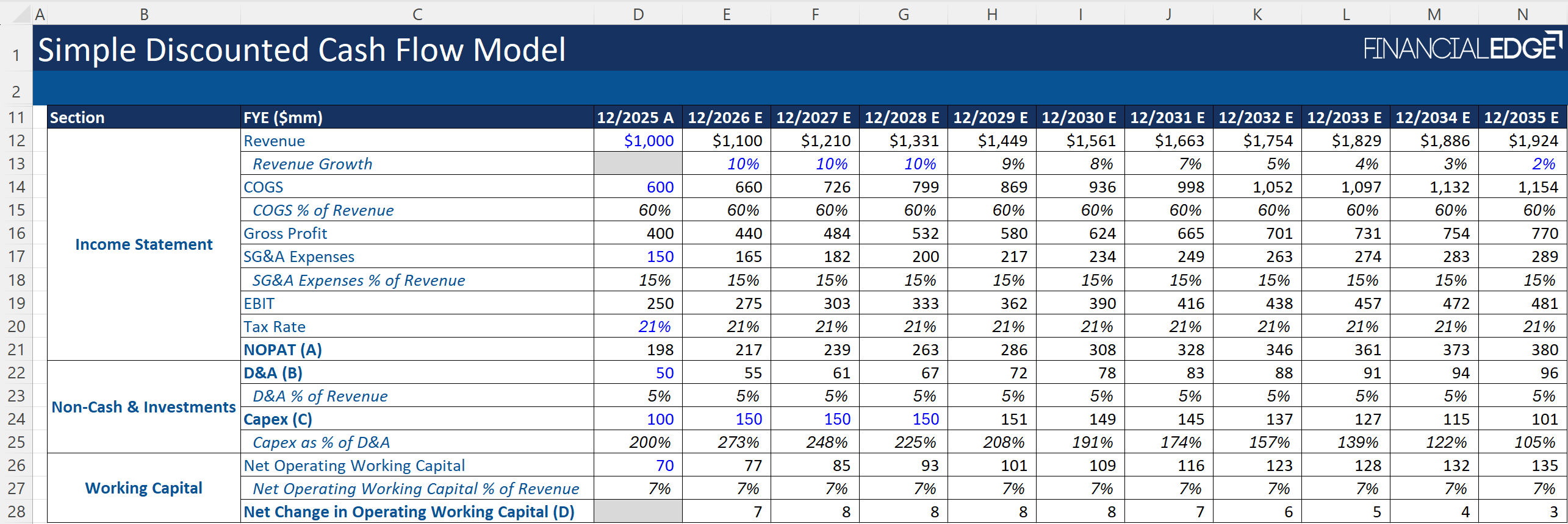
Step 2: Project the Income Statement, Non-Cash & Investments, and Working Capital

Future earnings are estimated by projecting line items based on historical margins and growth assumptions. This stage of the model translates the high-level assumptions into specific annual cash flows.

(Click to Zoom)

Income Statement

• Revenue: Calculated by applying a 10% growth rate for the first three years (through FY 2028), followed by a linear taper to 2% by FY 2035
• COGS (Cost of Goods Sold): Maintained at a constant 60% of revenue, reflecting the actual margins from FY 2025
• SG&A Expenses (Selling, General & Administrative): Maintained at a constant 15% of revenue, consistent with the FY 2025 actuals
• EBIT (Earnings Before Interest and Taxes): Derived by subtracting COGS and SG&A expenses from total Revenue
• Taxation: A standard corporate tax rate of 21% is applied
• NOPAT (Net Operating Profit After Tax): Calculated as EBIT times (1 – tax rate)

Non-Cash Expenses & Investments

• D&A (Depreciation & Amortization): Projected at a constant 5% of revenue, matching the FY 2025 actuals
• Capex (Capital Expenditure): Set at $150mm annually from FY 2026 to FY 2028. Post-2028, the Capex-to-D&A ratio, which begins at 225% (as of FY 2028), linearly tapers to 105% by FY 2035. The final Capex figure for each projected year is derived by multiplying this percentage by the respective year’s D&A

Operating Working Capital

• Net Operating Working Capital: Maintained at a constant 7% of revenue, consistent with FY 2025
• Net Change in Operating Working Capital: Calculated as the difference between the current year’s Net Operating Working Capital and the previous year’s. For example, if Net Operating Working Capital is $77mm for FY 2026 and $70mm for FY 2025, the Net Change in Operating Working Capital for FY 2026 is $7mm

Step 3: Calculate Free Cash Flow to Firm (FCFF)

FCFF is calculated as below:

(Click to Zoom)

• Add NOPAT (A)
• Add D&A (B)
• Subtract Capex (C)
• Subtract Net Change in Operating Working Capital (D)

Step 4: Determine Terminal Value and Total Enterprise Value

Using Gordon Growth Model, as described earlier in the blog, this step involves capturing the value of the company in perpetuity:

(Click to Zoom)

Timing Note: The Terminal Value of $4,750mm is calculated as at the end of the final forecast year i.e. FY 2035. Whether this figure represents the exact end of the year or a mid-year point depends on whether the mid-year convention is applied to the overall DCF model.

Step 5: Apply the Mid-Year Convention and Discounting and Calculate Enterprise Value

To account for the continuous flow of cash throughout the year, rather than assuming all cash is received in a single lump sum at year-end, the mid-year convention is applied to the discounting periods:

(Click to Zoom)

• Discounted Duration: Under the mid-year assumption, the duration for Year 1 is 5, Year 2 is 1.5, and the final year of the forecast period (Year 10) is 9.5
• Present Value (PV) Calculation: Using these adjusted durations, the PV is calculated for each specific forecast year
• Enterprise Value (EV): The aggregate of all individual discounted cash flows, combined with the discounted terminal value, results in a total EV of $3,352mm

DCF Analysis Pros & Cons

Pros

• Determination of Intrinsic Value: Unlike the Trading Comparables method, which relies on market multiples that can be skewed by market swings or irrational exuberance, a DCF provides a valuation based strictly on the fundamental cash-generating ability of the business
• Granularity and Transparency: The DCF framework is highly detailed. It allows an analyst to deconstruct the business and identify exactly where value is being created, whether through operational efficiency (margins), revenue growth, or disciplined capital allocation
• Sensitivity and Flexibility: The model serves as a dynamic tool. Any change in the business environment, such as a reduction in Capex requirements or an improvement in EBIT margins, can be instantly updated to reflect the impact on the company’s total value
• Universal Acceptance: The DCF is a globally recognized method. It is highly regarded by both equity investors and debt issuers as a rigorous method for evaluating long-term solvency and investment potential

Cons

• Heavy Reliance on Assumptions: The accuracy of the DCF is only as good as its inputs. From projecting revenue a decade into the future to estimating long-term operating margines and working capital needs, the model relies on a suite of assumptions about an uncertain future
• Complexity and Margin for Error: Because the model is so detailed, it is inherently prone to “garbage in, garbage out.” A small error in a single formula or an overly optimistic margin assumption can compound over the forecast period, leading to a significantly flawed valuation
• Sensitivity to Key Variables: The final output is highly sensitive to the WACC and Perpetual Growth Rate.

(Click to Zoom)

As highlighted above, shifting the WACC from 12% to 8% or adjusting the terminal growth rate by even 1% can cause the Enterprise Value to swing by 40% or more. This sensitivity means that a minor change in the discount rate can lead to very different investment conclusions

When Should You Use a DCF Model?

Capital Allocation and Strategic Planning: The DCF is an essential tool for internal decision making, particularly when evaluating capital budgeting projects. It allows managers to quantify the potential returns of long-term initiatives, such as launching a new product line or investing in a new production facility, to ensure they create value for the firm.

Fundamental Equity Valuation: For investment decisions, the DCF serves as the primary method for determining whether a company’s stock is undervalued or overvalued. By calculating the intrinsic value, investors can identify opportunities where the market price has significantly deviated from the company’s true fundamental worth.

Mergers, Acquisitions, and Negotiations: In the context of Mergers & Acquisitions (M&A), the DCF model is used to establish the intrinsic, stand-alone value of a target company. This figure acts as a critical baseline during negotiations, helping the acquiring party determine a fair purchase price before accounting for potential synergies.

Which Industries/Businesses are More Suited for a DCF Model?

While a DCF model can be applied to nearly any business by layering in the necessary assumptions, its reliability is highest when future cash flows are predictable. The model is best suited for stable, mature companies with consistent earnings and growth rates that are less susceptible to extreme market cycles or sudden technological disruptions. Industries such as utilities, infrastructure, mining, manufacturing, telecom, commercial real estate, and consumer staples, which often have long-term visibility into production or lease agreements or revenue flow, provide the steady-state environment where DCF projections excel. Conversely, high-growth sectors like technology, or early-stage startups are less suited for this method, as rapid innovation and shifting consumer habits can render long term growth assumptions obsolete very quickly.

Is Discounted Cash Flow Accurate?

The accuracy of a DCF is a double-edged sword. While it is mathematically precise, its real-world reliability is entirely dependent on the quality of its underlying assumptions.

• The Positives: The model’s strength lies in its transparency and granularity. It allows for a deep dive into value drivers like revenue growth, operational efficiency, and capital allocation. It is a dynamic tool that can be instantly updated to reflect changes in the business environment
• The Negatives: The model is highly sensitive to key variables, such as WACC and perpetual growth rate. Because it requires projecting financials a decade into an uncertain future, it is often prone to a “garbage in, garbage out” scenario where small errors compound into significant valuation flaws

In summary, a DCF is best used not as a definitive “crystal ball,” but as a powerful diagnostic tool to understand the conditions under which an investment becomes attractive.

Conclusion

The DCF model remains a cornerstone of financial analysis by providing a rigorous framework to determine a company’s Intrinsic Value. By focusing on the fundamental ability of a business to generate cash, rather than following volatile market trends, it allows investors and managers to make decisions based on long-term economic reality.

Additional Resources

Investment Banking Courses

M&A Explained

DCF Sense Check

Terminal Value

WACC

Free Cash Flows (FCF) – Unlevered vs Levered

Financial Accounting

3-Statement Model