Options Pricing Models

What are “Options Pricing Models”?

Option pricing models are theories that can calculate the value of an options contract based on the number of variables within the actual contract. The key aim of a pricing model is to work out the probability of whether the option is ‘in-the-money’ or ‘out-of-the-money when it is exercised.

There are several option pricing models such as the Black-Scholes Model (BSM) or Binomial Pricing Model which can be used to price options contracts. The former model is possibly the most well-known options pricing model. There are two distinct parts of an options price, namely its intrinsic value (which is a measure of the profitability of an option) and time value (which is based on the expected volatility of the underlying asset and time left until the expiration of the option – option contracts have a specified amount of time prior to their expiry).

There are two types of options – call options and put options. The option pricing models are used to calculate their pricing or value. These options grant a right, but not an obligation to a buyer to buy or sell the underlying asset. An important point to note is that an option is basically a derivative contract in which the buyer pays money to the seller (termed as the premium). Thereafter, in return, the buyer obtains the right to either purchase (a call) or sell (a put) a specified amount or quantity of an underlying asset at a fixed price (this is known as the strike price or an exercise price) either on a specific expiration date or on any day prior to the option’s expiration date.

Black-Scholes Pricing Model (BSM)

These two option pricing models (BSM and Binomial pricing model) are mathematical models to calculate the theoretical value of an option. They provide us with a fair value estimate of an option. This in turn helps investors to adjust their portfolios and strategies accordingly.

Options may be classified into European style (which can be exercised only at the option expiration date)  and American style (which may be exercised anytime between the purchase date and the date of options expiration). This classification is very important, as choosing between these two types of options will impact our choice of the option pricing model.

The BSM is a model which is widely used by options market participants and was developed primarily for pricing European-style options on stocks. It cannot be applied to American-style options.

The underlying assumptions of the BSM are that until the option expiration date, the stock will pay no dividends, the risk-free rate and variance rate (σ^2) of the stock are constant and known, and extreme changes in stock prices are ruled out. Further, this model assumes a normal distribution (bell-curve distribution) of continuously compounded returns.

Call Option – Black Scholes Pricing Formula

C = So N(d1) – Xe-rT N (d2)
d1= In (So/X) + (r + σ2/2)T/σ SQRTT
d2 = In (So/X) + (r – σ2/2)T/σ SQRTT = d1 – σ SQRTT
C = Current option value ( also called call premium)
So = Current stock price of stock A at time 0 i.e. price of the underlying asset
N(d1) and N(d2) = represent the standardized normal distribution probability that a random variable will be less than d i.e. d1 and d2 respectively.
X = Exercise price of the option – the price at which an option can be exercised
R = Risk-free interest rate (%)
σ = is the standard deviation or the price volatility, that is the volatility of returns of the underlying stock – i.e. it is a measure of how much the security prices will move in the subsequent periods.
SQRT = Square root
T = Time to the expiration of option or Time to Maturity  i.e. time between the calculation and an option’s exercise date
N = Normal Distribution

Having stated the above, we first have to calculate the values of d1 and d2.

The Black Scholes Model helps us to compute the call option price or value if we have the current stock price, exercise price, the risk-free rate, time to maturity, and the annual standard deviation of return of the underlying asset.

Next, the Black-Scholes model enables us to calculate the call option value or price and compare it with the current price of the option. One could buy the option if it is fairly priced.

It might be noted that the probability of exercising the call option increases, as the ratio of the current stock price to the exercise price increases.

Put Option – Black Scholes Pricing Formula:

P = Xe-rT N(-d2) – So N(-d1)
P = Price of Put Option

Binomial Option Pricing Model (BPM)

This is the simplest method to price the options. Please note that this method assumes the markets are perfectly efficient. In this model, we consider that the price of the underlying asset will either increase or decrease in the period. It values options deploying an iterative approach that utilizes multiple periods to value American options (where the holder has the right to exercise at any time up to expiration). Under the binomial model, the current value of an option is equal to the present value of the probability-weighted future payoffs from the options.

The BOPM is a popular tool for the evaluation of stock options. Investors use this model to assess the right to purchase or sell at specific prices over time. Further, the call option pricing and put option pricing or value using a one-period or multiple periods BOPM can be computed using formulas.

In essence, investors know (or can find out) the current stock price at any given moment in time and they attempt to guess what the stock price movements could be in the future. This model creates a binomial distribution of what could be the possible future stock prices. The price of the underlying asset (i.e. stock) will either go up or down in the period. This model is best represented by using binomial trees.

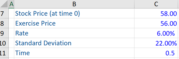
Black Scholes Model – Call Option Price and Put Option Price

Given below is an example of call and put option pricing using Excel. Here we have a 6-month call option (the right to ‘buy’ a stock) with an exercise price of US$56 on a stock whose current price is US$58, The r (risk-free rate) is 6% (this is in reality very high, but used here just as an example), σ or sigma (the annual standard deviation of stock returns) is 22% and T = 0.5 (i.e. it is a six-month call option so ½ a year).

The call price calculation involves 5 steps: the first step is to calculate d1, followed by calculation of d2, N(d1), N(d2), and finally the computation of the call price (US$5.61). The probabilities for N ( ) are estimated with the Norm.S. Dist function.

It might be noted that N(d1) and N(d2) represent approximately the probability that the exercise price of the option will be greater than the current stock price.

After the calculation of the call option price following the aforesaid steps, the put option price is calculated (US$1.95)