
Test Yourself
Sign up to access your free download and get new article notifications, exclusive offers and more.

How to Build a Financial Model
August 6, 2021
What is “Financial Modeling?”
Financial modeling refers to a process that is used to forecast a company’s financial performance over a specific period of time (for example, 3 or 5 years). There are usually four components to this forecasting task:
- Inputting publicly available or private historical data – the financial model’s projections are typically based on the historical financial performance of the company.
- Constructing ratios and statistics predicated on this historical data – for example, historical data on sales.
- Making future assumptions – for example, if historical sales have gone up 10% every year, this assumption can continue into the projection period.
- Forecasting financial data based on assumptions – for example, if Year 0 sales were $100, this year’s sales would be $110.
The forecasting process necessitates the preparation of the company’s financial statements – balance sheet, income statements, and cash flow statements – and the supporting schedules. The data is typically inputted into Excel, using a series of hard-coded entries and simple formulas to find totals or calculate certain data points. Thereafter, models such as Discounted Cash Flow (DCF), Sensitivity Analysis, Leveraged Buyout (LBO), etc. can be constructed from the data gathered.
Key Learning Points
- The forecasting process has four components – inputting historical data, constructing ratios and statistics, making future assumptions, and forecasting financial data.
- The modeler, when constructing a financial model, has to choose between several design choices to lay out the data.
Financial Modeling Structure – Design Choices
The modeler has many choices to make when constructing a financial model, including how many Excel sheets to use, where to put the model assumptions and how to format the negative numbers. For smaller models, a single Excel sheet is ideal (a DCF model is commonly built using a single sheet). For more complex models and larger companies, a multiple sheet structure is preferable.
A more detailed design choice involves the treatment of forward assumptions, which drive the model output. The options are to group all the forward assumptions in one specific area in the model. The benefit is that this is user-friendly, even in a large model. However, some modelers prefer to have the assumptions (of revenue growth, operating income & costs, and taxes as % of profit before tax) spread throughout the output, since it means that both the driver and the result can be seen at the same time. It is important to be consistent when using negative figures or cash outflows so that they aren’t misused or misread in future calculations.
Financial Modeling Example
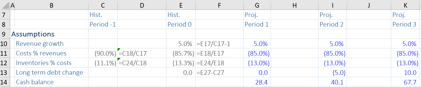
Given below is an example of financial modeling, where the income statement and balance sheet for the forecast period are built using historical data. From there, some ratios and statistics are calculated (including Revenue Growth, Costs as % of Revenues, Inventories as % of Costs, and Long-Term Debt Change). These metrics can support the rationale for deriving forecast assumptions for the income statement and balance sheet from the year (period) 1 to 3. Next, we use these forecast assumptions to calculate the forecast figures for the income statement and balance sheet accordingly. Typically, this can be done by linking the excel cells of historic data with the forecast growth data to calculate the future estimates.
Forecasting the Income Statement
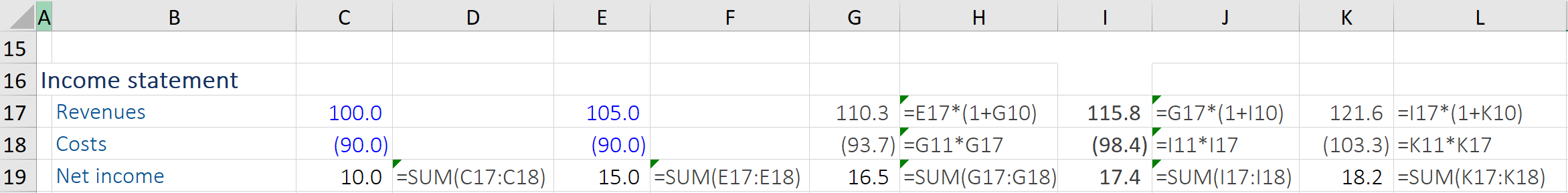
To calculate the revenues for the forecast period, we will multiply the last (historical) year’s revenue with the following year’s revenue growth assumption (5%) and so on to get forecast revenues. This can be linked up using the Excel formula, ideally without any hard-coded figures so the model will accurately reflect any changes in assumption or new historical data when added.
In the table below, we see the Cost as % of Revenues assumption of 85% (i.e. 85% of 110.3 (Revenue) and similar ratios to get the forecast costs. We can then calculate the net income for the forecast period. Net income (on the income statement) of the historical period has to also be computed (i.e. Revenues – Costs).
Balance Sheet Forecasting
For the historic data, the total assets on the balance sheet has to be calculated too (this is usually Cash + Inventories = Total Assets), which is demonstrated below. The sum of total liabilities on the balance sheet has to be computed.
Moving down to the balance sheet, the cash assumption is already given. For the calculation of inventories for the forecast period, we can use the inventories as a % of costs ratio (13% in this case) and multiply it by the costs in the forecast years (period 1 to 3). Adding these up, we get the total assets for the projected years.
Lastly, we want total assets to be equal to total liabilities and equity. To arrive at total liabilities, we compute long-term debt for the forecast period, using the long-term debt year-over-year change assumption (in this instance 0%, so no change from last year for the first projected year). In this example, there is no specific assumption for equity. So, we take the net income from the income statement and add it to last year’s equity (i.e. 16.5 + 14 = 30.5), and so on. In all forecast years, the balance sheet ought to balance.
Finally, with all financial modeling, it is sensible to check that all the data entries and forecasts are complete (and that formulas remain correct throughout), and that the balance sheet ‘balances’ as per the ‘check’ line below.
Additional Resources
Learn to build financial models with our online financial modeling course. Our online courses will teach you everything you need to know to succeed.