Post Match Workout
Send download link to:
Featured Product

MATCH Function
January 14, 2021
What is the MATCH Function?
According to Excel =MATCH “Returns the relative position of an item in an array that matches a specified value in a specified order”. Practically speaking, it finds the position of a cell within a range of cells.
The key thing to note with MATCH is that it returns a number. It is similar in many respects to =VLOOKUP, especially with regard to syntax options, but whereas VLOOKUP returns the contents of the found cell (item) MATCH returns the position of the cell – a numeric value relative to the start of the range (array).
Key Learning Points
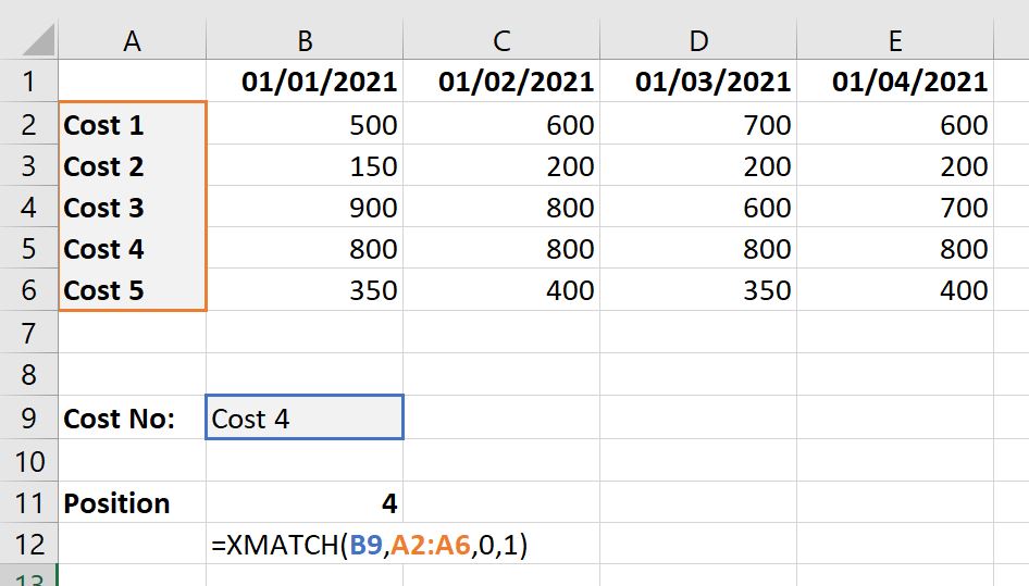
- The MATCH function returns the relative position of the cell from a range of cell as a numeric value
- The lookup value entered into the MATCH function can be hardcoded but it is best practice to link to a separate cell
- The MATCH function is commonly used in conjunction with the VLOOKUP function to make the col_index_num in VLOOKUP dynamic
- XMATCH performs the same function as MATCH but is much more powerful and includes a search mode and match mode for increased usability
Syntax
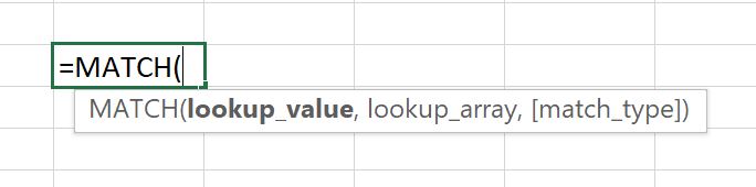
=MATCH( lookup_value , lookup_array , [match_type] )
Lookup_value: The value to be found. This can be hard-coded but is more likely to be a cell reference.
Lookup_array: The range of cells (array) to look in.
[Match_type]: Optional. One of three options (exactly like VLOOKUP)
- 1 (Default if omitted) = Less than: Finds the largest value in lookup_array that is less than or equal to lookup_value. For this to work lookup_array must be in ascending order.
- 0 = Exact match: Finds the first occurrence of lookup_value in lookup_array that is exactly equal. Lookup_array can be in any order.
- -1 = Greater than. Finds the smallest value in lookup_array that is greater than or equal to lookup_value. For this to work lookup_array must be in descending order.
Notes:
- Lookup_array must be only 1 row tall or 1 column wide. Any more and the #N/A error will be given.
- The most commonly used match_type is 0 (exact match) because lookup_array can be in any order. The other two options are very useful but only in limited circumstances, and have an extra danger if the data in lookup_array changes and is no longer in the necessary order. So, care must be taken when using these other two options.
- When lookup_value is a number (recognised by Excel as a number) then the values in lookup_array must also be numeric otherwise a match won’t be found.
- Wildcards * and ? (and ~) can be used as part of text-based searches.
Example
Because MATCH returns a number, a common use of MATCH is in conjunction with VLOOKUP, to make the col_index_num in VLOOKUP dynamic. This blog does not cover VLOOKUP in detail.
=VLOOKUP(lookup_value , table_array , MATCH( lookup_value , lookup_array , [match_type] ) , [range_lookup])
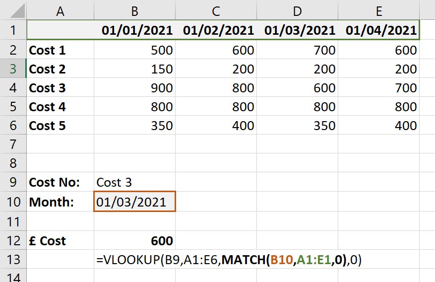
In this simple example the use of MATCH allows both the row to by dynamic, because of the VLOOKUP, and also the column because of the MATCH. A different month can be entered int cell B10 to get the result from a different month. Using this combination of VLOOKUP and MATCH makes the whole data table accessible dynamically.
The only note of importance when using this combo is that the start column of both ranges must be the same, in this case column A.
=VLOOKUP(B9,A1:E6,MATCH(B10,A1:E1,0),0)
This is to ensure that col_index_num returned by the MATCH portion is correct for the rest of the VLOOKUP. If this is not possible then an adjustment must be made to the MATCH formula, by appending plus or minus numbers to it.
Download the accompanying Excel file to look at some examples.
XMATCH
In 2019 Excel announced a series of new functions. These have become available to users since then, depending on which version of Excel you have. One of those new functions is XMATCH. On the surface it appears to be similar to MATCH, but it is actually much more powerful.
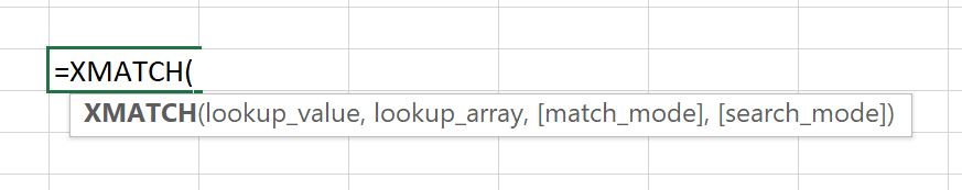
=XMATCH(lookup_value , lookup_array , [match_mode] , [search_mode])
Lookup_value and lookup_array: as before
[Match_mode]: Optional. One of four options
- -1 = Exact match or next smaller item: Attempts an exact match first and if not found then returns the next smallest.
- 0 (Default) =Exact match: As before
- 1 = Exact match or next larger item: Attempts an exact match first and if not found then returns the next largest.
- 2 = Wildcard character match: There appears to be very little actual explanation as to what this option actually does, even on the Microsoft website! From what we can gather, it allows the use of wildcards as part of lookup_value, however in our testing the same results were sometimes obtainable using match_mode of 1 but still with wildcards in lookup_value!
[search_mode]: Optional. Again, one of four options
- 1 (Default) = Search order first-to-last
- -1 = Search order last-to-first
- 2 = Binary search (lookup_array must be in ascending order)
- -2 = Binary search (lookup_array must be in descending order)
Notes:
- Remember that XMATCH returns the position of lookup_value in lookup_array, not the contents of the cell.
- Even with match_mode as 1 or -1, the data in lookup_array does not need to be in order (as long as search_mode is either 1 or -1)
- Because, like VLOOKUP, XMATCH returns the first instance of the found result, using search_mode = -1 is very useful to find the last occurrence of something.
XMATCH Example
Microsoft have designed XMATCH to be a direct replacement for MATCH. Therefore, for a lot of situations the application of XMATCH is exactly the same as it would be for MATCH. In this example of XMATCH you could just as easily use MATCH!